This vignette purposes is to show users how to use stackr to run the stacks pipeline inside R/RStudio.

stackr assumptions

stackr is similar to stacks concerning data quality: it won’t make your sequencing data better. Bad input data is just that… bad!
You have read stacks manual and understand the separate modules and the outputs that stacks produces.
You have read the latest stacks paper (version 2, Rochette et al. 2019):

stackr advantages

Run stacks inside R/RStudio/RStudio Server. If you don’t like R, stackr is not the tool for you.
The philosophy of working by project with pre-organized folders.
stackr is not slowing down stacks it’s actually making some steps faster with parallelization.
If you have > 1 sequencing chip/lane: this workflow will save you a lot of time.
Technical replicates: inside or across chip/lanes are managed uniquely (you want technical replicates…).
Noise reduction.
Data normalization.
Crashing computer/cluster/server ?:
- stackr is also on my Amazon AMI
- no more nightmares of having to restart your stacks pipeline because of a crashed server… stackr manage stacks unique integer (previously called SQL IDs) throughout the pipeline. It’s integrated from the start, making it a breeze to just re-start your pipeline after a crash!
mismatch testing: de novo mismatch threshold series is integrated inside run_ustacks and stackr will produce tables and figures automatically.
catalog: for bigger sampling size project, breaking down the catalog into several separate cstacks steps makes the pipeline more rigorous if your computer/cluster/server crash.
logs generated by stacks are read and transferred in human-readable tables/tibbles. Detecting problems is easier.
summary of different stacks modules: available automatically inside stackr pipeline, but also available for users who didn’t use stackr to run stacks.
Detecting problems is easier.
Increased reproducibly.

Coding style

stackr is trying hard to follow the tidyverse style guide.
inside stacks, parallel execution and the use of threads sometimes uses the argument -p, -t, --threads. Depending on module the meaning changes, which can be confusing or generate problems for first-time users. Inside stackr, using parallel execution is always through the use of the argument: parallel.core.
argument break down inside stacks modules sometimes uses the hyphen -. Inside stackr this is replaced by function arguments with . point/dot. Example: in stacks process_radtags argument --adapter-1 will be the argument adapter.1 inside stackr run_process_radtags.

Workflow

The names of stackr functions follows stacks module, below the similarity:

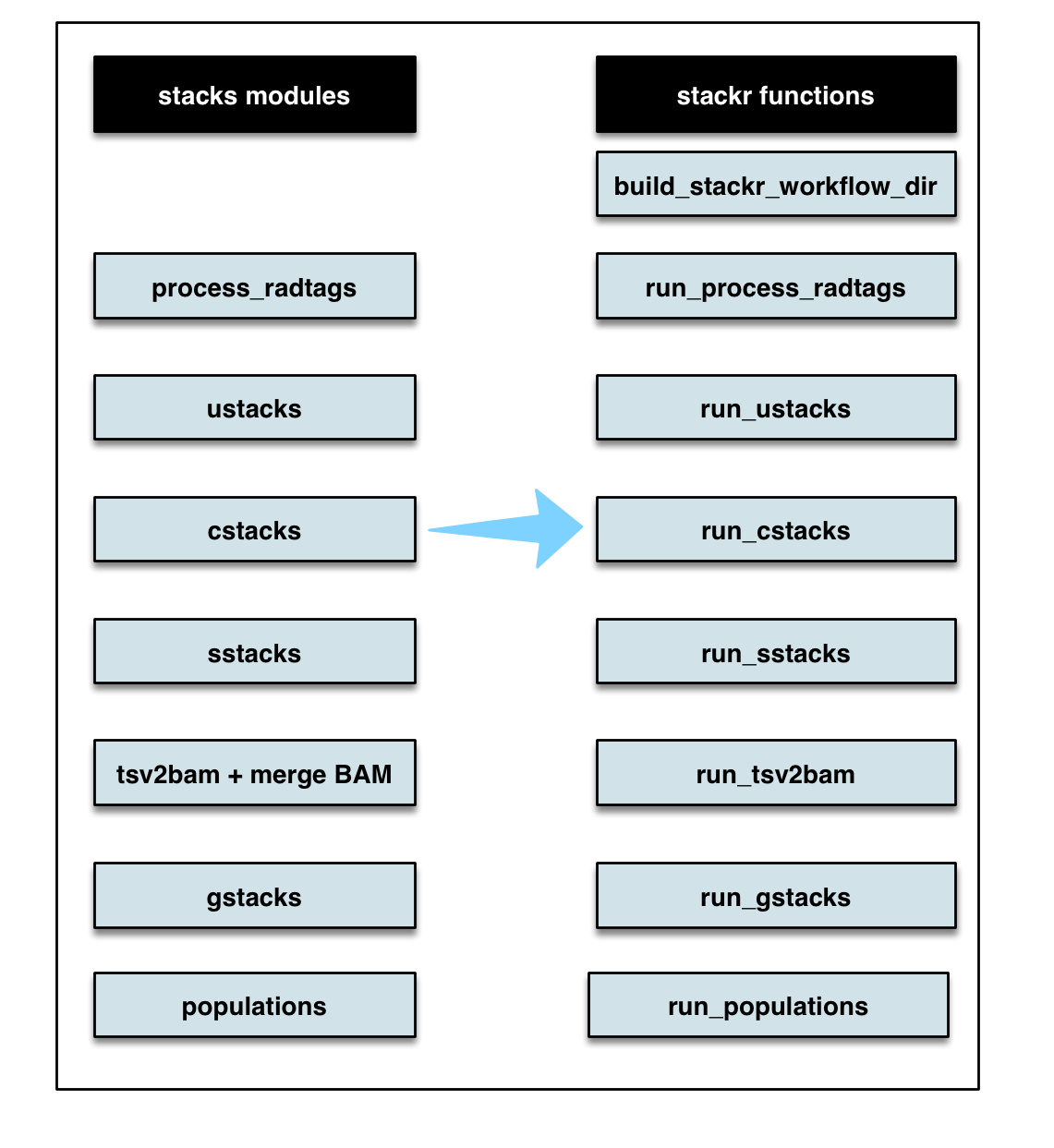
They are tons of other workflows and below are just a few examples:

Dependencies

Make sure you have the latest R and RStudio version before installing stackr. My other package radiator as a nice vignette for this.
Install stacks and it’s dependencies (my own installation pipeline here).
don’t write to me if you’re having problem at this step.
stacks google group is your best friend.
Install stackr by following the instructions.

Generate project folders

Here, I’m going to use RStudio, because I really got to like it and I’m very efficient in it. But it’s by no mean essential.

Set your working directory inside RStudio using setwd function and appropriate path.
Generate the folders for your project

To get the doc on the function we’re about to use: ?stackr::build_stackr_workflow_dir.

Let’s start a project on turtles…

stackr::build_stackr_workflow_dir(main.folder.name = "turtle")
# stackr::build_stackr_workflow_dir(main.folder.name = "turtle", date = FALSE) #if you don't want the date appended

By default, the date and time is appended to the main folder and inside, these folders will be generated:

01_scripts
02_project_info
03_sequencing_lanes
04_process_radtags
05_clustering_mismatches
06_ustacks_2_gstacks
07_populations
08_stacks_results
09_log_files
10_filters

For now let’s just say that you put the scripts and other .R files associated to this project inside the first folder: 01_scripts.

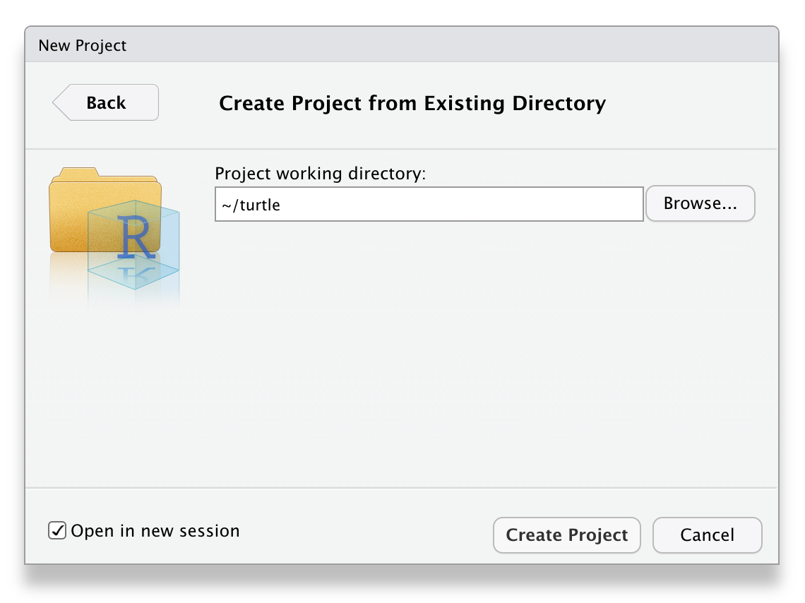
Start a project

Inside RStudio generate a new project inside the directory just created:

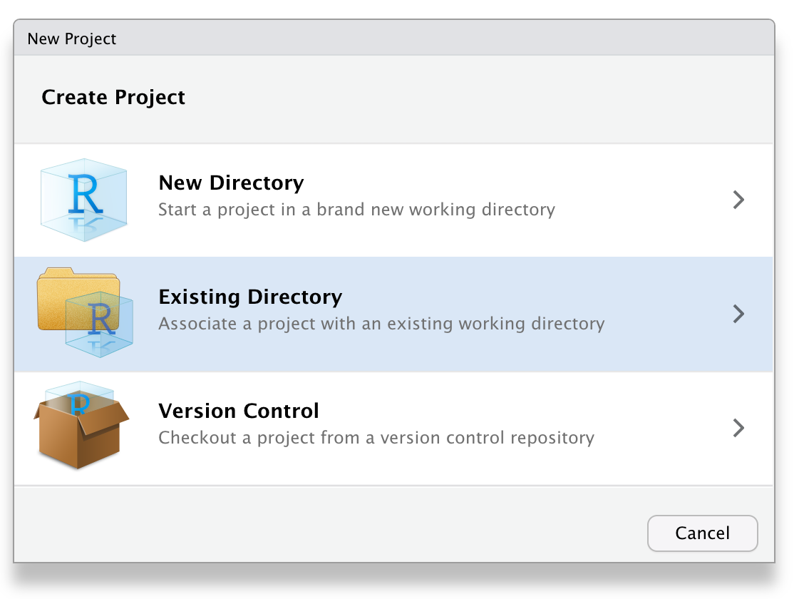
You can add the alias/shorcut for the project on your computer desktop.

Project info file

Inside MS Excel or another software that works with tabular columns, prepare your project info file and save it with the file extension .tsv inside the second folder: 02_project_info. For example, the file project.info.turtle.tsv will contain a minimum of 3 columns for single-end and 4 columns for paired-end sequencing. The number of lines equal the number of sample: 1 sample per line. The project info file is sample oriented or focused.

But before generating and filling the project info file consider the names of your samples…

The art of naming your samples

You already have somewhere on your computer barcodes and sample name. Here is the time to reconsider how you named your sample. This is not trivial, researcher loose a lot of time because of bad naming scheme. REALLY.

My philosophy:

Include useful metadata associated with your sample separated by an hyphen -. Why an hyphen - instead of a point . or an underscore _ ?? Imagine you print your file on real paper or that you have to translate by hand the sample names. An hyphen, when printed, generated far less confusion because it can easily be distinguised if printed on paper (lined paper or not). The underscore or point will just be confusion with space.

Please don’t use space
Please use ALL CAPS so that confusion is minimized.
The key here is consistency.

Below an example using metadata: SPECIES, STRATA (could be location, I don’t know the pop yet), YEAR (of sampling), SEX, ID (with sufficient digits)

STU-BUR-2019-F-0001
STU-BUR-2019-F-0002
STU-BUR-2019-F-0003
STU-BUR-2019-F-0004
STU-BUR-2019-M-0005
STU-BUR-2017-F-0006
STU-GRA-2017-M-0007 # you could start over from 0001 with different strata, it doesn't matter
STU-GRA-2018-M-0008
STU-GRA-2019-M-0009
STU-GRA-2019-F-0010
STU-GRA-2019-F-0011

Special considerations:

keep it simple.
you can use 3 or 4 letters for the metadata, but inside 1 metadata but please please be consistent.
future parsing, if you need it, will be very very easy this way.

Ok now the project info file…

single-end

Columns prerequisites:

LANES: the name of the sequencing file e.g. H6CY7BBXY_3_254.fastq.gz
BARCODES: the barcode associated with the sample.
INDIVIDUALS: a more appealing sample name (more on this below).

Generate an empty file like this:

tibble::tibble(
  LANES = character(0), 
  BARCODES = character(0), 
  INDIVIDUALS = character(0)
) %>% 
  readr::write_tsv(x = ., path = "02_project_info/project.info.turtle.tsv")

paired-end

Columns prerequisites:

BARCODES: the barcode associated with the sample
INDIVIDUALS: a more appealing sample name (more on this below)
FORWARD: the name of the forward sequencing file e.g. H5CY5BBXY_2_25_1.fastq.gz
REVERSE: the name of the reverse sequencing file e.g. H5CY5BBXY_2_25_2.fastq.gz

Generate an empty file like this:

tibble::tibble(
  BARCODES = character(0), 
  INDIVIDUALS = character(0),
  FORWARD = character(0),
  REVERSE = character(0)
) %>% 
  readr::write_tsv(x = ., path = "02_project_info/project.info.turtle.tsv")

FAQ

Multiple sequencing lanes or chips ?

If you have several Illumina lanes or Ion Torrent chips, just write them down along the sample and barcodes associated with it. On the same file.

Technical replicates ?

2 options:

use separate name for it or best,
let stackr manage it my using the same name (yes… yes…).

stackr will see that you have, for different barcodes/lanes combo, ids that have the exact same name. What will happen ?

things will be kept separate and -1 and -2 will be added to the sample name.
after run_process_radtags, the replicates will be combined and the new file will have -R at the end. The individual replicates are kept separate as well.

example:

You have a sample, STU-BUR-2019-F-0001, on 2 separate wells on the the plate or even lanes, with different barcode. At the end of run_process_radtags you’ll have:

STU-BUR-2019-F-0001-1
STU-BUR-2019-F-0001-2
STU-BUR-2019-F-0001-R (for the combined replicates)

No lanes just individual’s fq files ?

Example: you used DArT sequencing services. You have individual fq files, the barcodes are still in there along some Illumina adapters.

Use the LANES column for the individual FQ files that requires to go through stacks process_radtags.

Transfer sequencing files

Transfer the sequencing files inside the folder: 03_sequencing_lanes. Contrary to the pipeline I used to contribute and follow link Don’t modify the files: stackr, like stacks, handles the different types.

Quality control

I highly recommend running the sequencing files (entire lane or chip) through a software dedicated for QC. If you have bad sequencing, no need to go further in the pipeline…

FastQC.
fastqcr is the R alternative.

run_process_radtags

This is the demultiplexing step in stacks, the module is called process_radtags.

Function documentation: ?stackr::run_process_radtags (read it twice).

Note:

I really like cutadapt, it’s my working horse for reads operations. However, I no longer recommend, using it, unless you have very very problematic fastq files or need to do very specific operations on your reads. Stay with stacks, process_radtags will handle your fastq files just fine.

Difference with stacks process_radtags ?

You have one function that will run all you lanes/chips.
Technical replicates will be managed and combined.
A summary of the process will be generated.

The function will generate, inside 08_stacks_results, files like these:

process_radtags_LANE_01_barcodes_stats.tsv
process_radtags_LANE_01_stats.tsv

These files have the statistics per barcodes and per lanes. The logs are found inside the folder: 09_log_files.

The project info file will be populated with these columns/info:

TOTAL: the number of total reads.
NO_RADTAG: the number of reads without radtags.
LOW_QUALITY: the number of reads discarded because of low quality.
RETAINED: The number of reads retained after the filters used inside process_radtags.
SQL_ID: A unique integer that will be used inside the next step: run_ustacks
FQ_FILES_F: the individual forward fq files
FQ_FILES_R: the individual reverse fq files

reads length

If you are using Illumina sequencing, chances are that you have 100 pb reads (SE RADseq). With Ion Torrent, the size will be highly variable and you have to determine the optimal size to cut your reads to the same length (stacks works better with uniform read length, check stacks manual under section Sequencer Type).

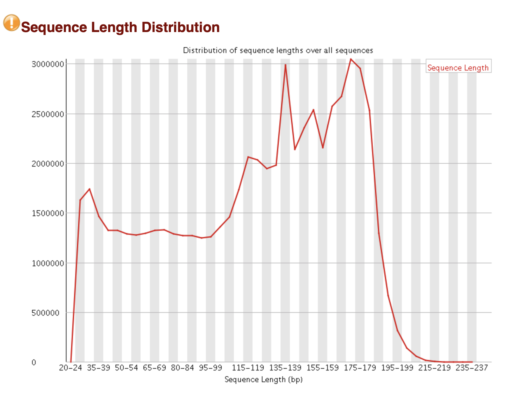
output of FastQC

FastQC will output the read length distribution. But it’s difficult to know how many markers you will get depending on read size.

You will see the relationship between the position of the nucleotide on the read and overall quality. This is very helpful to determine if you want to cut all your Illumina reads to 80 or 90 pb.

Below is a FastQC figure of a typical Ion Torrent sequencing chip sequence length distribution:

Use stackr

Below is a figure generated by stackr that shows the number of reads you will get depending on the maximum size threshold selected:

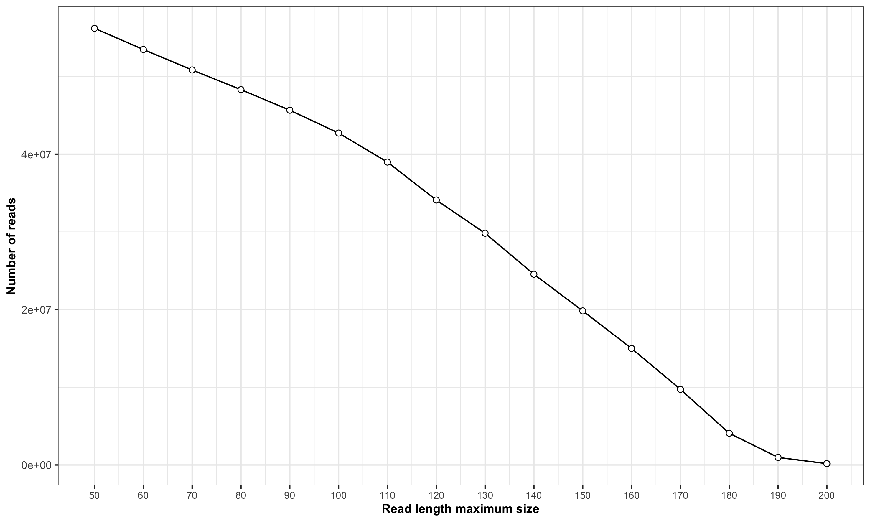
The function is:

size <- stackr::reads_length_distribution(
  fq.file = "my-fastq.fastq.gz", 
  with.future = TRUE, 
  parallel.core = 12L
  )

You can use individual file or entire chip or lane. Function documentation: ?stackr::reads_length_distribution

Remember that depending of types of file (individual or entire lane/chip:

Barcodes and adapters might be in this relationship observed in the figure.
It’s not uncommon to see increasing adapters present with increasing read size.
Repetitive sequences, unique reads and so on might impact the results (see noise section below).

SE RADseq

Example with single-end, 2 enzymes RADseq//GBS data:

step1 <- stackr::run_process_radtags(
  project.info = "02_project_info/project.info.turtle.tsv",
  path.seq.lanes = "03_sequencing_lanes",
  q = FALSE,
  renz.1 = "pstI", 
  renz.2 = "sphI",
  t = 90, 
  len.limit = 90,
  filter.illumina = TRUE, 
  retain.header = TRUE,
  adapter.1 = "CGAGATCGGAAGAGCGGG", 
  adapter.mm = 2,
  parallel.core = 12
)
# look for the remaining default arguments...

PE RADseq

Example with paired-end 1 enzyme RADseq:

step1 <- stackr::run_process_radtags(
  P = TRUE,
  project.info = '02_project_info/project.info.turtle.tsv',
  path.seq.lanes = "03_sequencing_lanes",
  enzyme = "sbfI",
  adapter.1 = "CGAGATCGGAAGAGCGGG",
  adapter.2 = "CGAGATCGGAAGAGCGGG",
  adapter.mm = 2,
  t = 90, 
  len.limit = 90,
  retain.header = TRUE,
  parallel.core = 8
)
# look for the remaining default arguments...

QC

I highly recommend running the individual fastq files through FastQC or fastqcr.

Noise reduction

Reducing the noise in an individual FQ file could really help speeding up your analysis. I use it when I have more than 200 samples. Nothing new here:

Daniel Ilut explains it in his pipeline (Ilut et al. 2014) and my function here his basically the same as his but in R…
Jon Puritz’s dDocent data reduction step as a similar example.
Praveen’s pipeline RADProc (Ravindran et al. 2019) use something similar.
Metagenomic analysis pipeline all have some step of denoising the data.

Visualization

I prefer Daniel Ilut way of visualizing the information.

The function stackr::read_depth_plot requires 1 FQ file (after stacks process_radtags or stackr::run_process_radtags) and is very fast to run. It will highlight read coverage groups of distinct reads within a sample. When I say distinct reads, is reads that are exactly the same, no mismatches. The distinct reads are putative allele.

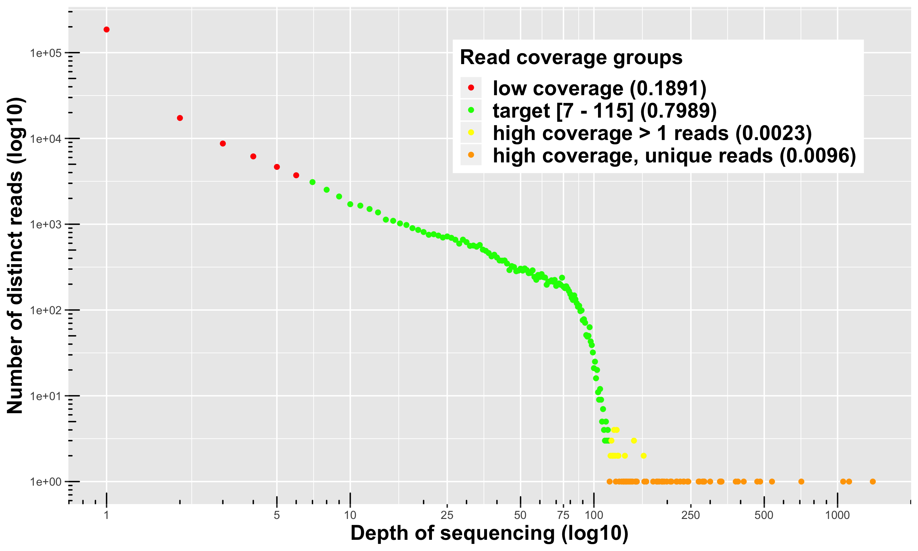
4 read coverage groups are shown:

distinct reads with low coverage (in red): these reads are likely sequencing errors or uninformative polymorphisms (shared only by a few samples).
disting reads for a target coverage (in green):
- Usually represent around 80% of the reads in the FQ file.
- It’s a safe coverage range to start exploring your data (open for discussion).
- Lower threshold (default = 7): you could go as low as maybe 3 ? You can’t escape it, it’s your tolerance to call heterozygote a true heterozygote. You want a minimum coverage for both the reference and the alternative allele. Yes, you can use population information to lower this threshold or use some fancy bayesian algorithm.
- Higher threshold: is a lot more open for discussion, here it’s the lower limit of another group (the orange, see below for description). Minus 1 bp.
distinct reads with high coverage > 1 read depth (in yellow): those are legitimate alleles with high coverage.
distinct and unique reads with high coverage (in orange): this is where you’ll find paralogous sequences, transposable elements and other high copy number variants.

To run it on your data:

read.plot <- stackr::read_depth_plot(
  fq.file = "04_process_radtags/my-fq.fq.gz",
  min.coverage.fig = 7L, #default
  parallel.core = parallel::detectCores() - 1 #default
)

The function will generate the plot shown above and write the figure in the working directory, using the sample name: my-fq_hap_read_depth.png.

FAQ

Should I run the function on all samples ?

Please don’t. Their is no use in running this on the entire dataset. It’s going to be fairly the same. Run it on a couple of samples. Based on the number of reads (distribution), choose 1 sample: below average, average and above average and compare the look of the figures produced.

Filtering ?

Removing the noise in FQ files, it’s usually a hot topic… Personally, the less I do the better and it’s definitely the case for small projects. I don’t think the noise is a problem for stacks. For large projects, it’s something else, and certainly a huge bottleneck. When you generate de novo assembly for more than 200 samples and generate a catalog with all the noise, cleaning the data can represent weeks of computation time that you shave off your project… really.

You don’t have to believe what I just wrote, test it yourself:

1. Clean the FQ file

Use the sample you just used in the read coverage groups, above, clean it with stackr::clean_fq. It’s very fast to run:

clean.fq.name <- stackr::clean_fq(
  fq.file = "04_process_radtags/my-fq.fq.gz", 
  min.coverage.threshold = 2, 
  remove.unique.reads = TRUE, #default
  write.blacklist.fasta = TRUE,
  write.blacklist = FALSE, #default
  parallel.core = parallel::detectCores() - 1, #default
  verbose = TRUE #default
  )

This will generate:

my-fq_cleaned.fq.gz # the cleaned fq file
my-fq_blacklisted_reads.fasta.gz # a fasta file with blacklisted sequences...

2. de novo assembly

Run stacks ustacks or even better, stay in stackr and do the next step below: the mismatch threshold series (using stackr::run_ustacks). For this, use the raw and clean FQ files and compare the output…

In all my projects, having less reads (the cleaned FQ file) means:

faster de novo assemblies (I’ve seen up to 3 times faster).
less loci generated, but of better qualities:
- higher coverage in all the de novo assembly steps of stacks
- less repetitive stacks blacklisted
- lower number of locus with assembly artifacts (lors of SNPs/locus, etc)
- very similar heterozygosity and homozygosity proportions
the mismathches plots are almost always identical: showing me that I can use the same Mismatch threshold (the -M in stacks ustacks) for the cleaned or the raw FQ files.
faster catalog generation time, the stacks cstacks or stackr::run_cstacks step.
NO DIFFERENCES in downstream analysis (population structure, outlier detection, Fst, assignment, closekin).

Why keep the blacklisted sequences (the fasta file) ?

You could use Biostrings::countPattern function to look for TE in those sequences;)

3. Filtering the entire dataset

If you see a big difference and are convince that filtering is the way to go, you can easily do it with this piece of code:

fq.to.clean <- list.files(path = "04_process_radtags/")
names(fq.to.clean) <- fq.to.clean

clean.all <- purrr::map_df(
  .x = fq.to.clean, 
  .f = stackr::clean_fq,
  min.coverage.threshold = 5, 
  remove.unique.reads = TRUE, #default
  write.blacklist.fasta = TRUE,
  write.blacklist = FALSE, #default
  parallel.core = 12
)

Transfer the cleaned files or the raw ones in a separate folder/sub-folder to keep things tidy.

Data normalization

Another hot topic, up for debate…

After the stacks step called process_radtags, in stackr run_process_radtags, looking at the distribution of the number of reads per sample, you might be getting one of these distribution:

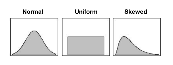
In an ideal world, you want the uniform distribution. That translate in good field and wet-lab techniques:

tissue sampling and preservation
extraction (robots ?)
pipetting
DNA quantification
all the other required techniques

And this resulted in similar sequenced information between your samples. You’re about to compare apples with apples. :)

If you have a skewed (left or right) or a normal distribution, you’ll be comparing apples with … citrus. The samples with lower reads will have less loci and usually less heterozygous loci. Similarly, the samples with higher number of reads will have more loci, more heterozygous loci.

What’s the likely cause for these ?

student with no prior wet-lab experience doing the DNA extraction or downstream step (e.g. library prep)
data preservation issues: historical DNA, fragmented DNA, etc.
skipping the DNA quantification or library QC steps

Ok, but what’s the problem with that ?

Potentially these problems:

ascertainment bias that could drive populations polymorphism discovery bias
missing data patterns
individual heterozygosity problems or patterns
downstream analysis impacted by the differences between your samples: artifactual or biological ?

Solutions ?

1. Wet-lab normalization

Here are the basic steps:

sequence the samples
look at the stats we’ve discussed
go back in the wet-lab to prepare a new plate
sequence
pool or not the lanes/chips
look at the sequencing statistics
repeat the step above or continue with the pipeline

I’m not a fan:

Way to many wet-lab steps.
The wet-lab is THE MOST important part.
Everything gets exacerbated with RADseq.
I’m not in favor of pooling lanes or chips (more on this some day!).
It’s really not like working with microsatelites.

2. Bio-informatic normalization

When doing it right from the start is impossible, I prefer to do the normalization after de demultiplexing step… after stackr::run_process_radtags. The prerequisite is to have enough sequencing material (reads) for all my samples.

The tool? stackr::normalize_reads function.

Rarefaction of fasq files by sub-sampling the reads before de novo assembly or alignment is not new:

Community and biodiversity ecologists are well aware of species accumulation curves obtained with rarefaction (Sanders, 1968). The rarefaction method guarantees the samples have the same weight in the analysis.
Metagenomics community before analyzing the alpha diversity will deal with differing sample depth for a given diversity statistic by using rarefaction. It means taking a random subset of a given size of the original sample (see mothur, Schloss et al. 2009).
Molecular ecologists for some reasons, RADseq enthusiasts seems unaware of this concept, but see (Hale et al. 2009; Kalinowski, 2004 and Puncher et al. 2018).
The Keywords: rarefaction, sub-sampling, normalization, standardization, sample size correction.

The steps ?

the goal is to reduce variance in number of reads between samples
rarefaction/normalization is conducted aon the fq file after stacks process_radtags and after removing the noise.
normalized replicates are generated by the function by randomly selecting the reads (without replacement) for each samples
you choose the number of replicates (default: 3) and you manage those replicates like other replicates you might have (you want replicates…).

Read the function documentation and look at the example

# To run this function, bioconductor's ShortRead package is necessary:
source("http://bioconductor.org/biocLite.R")
biocLite("ShortRead")

# Using OpenMP threads
nthreads <- .Call(ShortRead:::.set_omp_threads, 1L)
on.exit(.Call(ShortRead:::.set_omp_threads, nthreads))

# using defaults:
stackr::normalize_reads(path.samples = "~/corals")

# customizing the function:
stackr::normalize_reads(
   project.info = "project.info.corals.tsv",
   path.samples = "04_process_radtags",
   sample.reads = 2000000,
   number.replicates = 3,
   random.seed = 3,
   parallel.core = 12
   )

My observations using rarefaction:

the replicates have similar mismathches plots: showing me that I can use the same Mismatch threshold (the -M in stacks ustacks) for the rarefied samples.
better de novo assembly statistics
when the individual or population heterozygosity is a real biological signal, rarefaction doesn’t impact the downstream analysis.
when the heterozygosity was driven by the sequencing bias, bioinformatic rarefaction took care of the problem.

FAQ

It doesn’t bother you to throw away all the valuable information that samples with high read numbers have ?

Absolutely not!

most of the information is already lost: that is if you used stacks to generate a catalog and then filtered the data to keep markers in x individuals and/or in all sampling sites/populations. At this step it’s either you loose markers or get more missing data…
It’s not a loss of information if the information cannot be confirmed with other samples: it’s a statistic problem and ecologists are well aware of this.
The loss of reads is intrinsic to RADseq: Don’t believe me, inspect stacks, stackr or any RADseq pipeline log files… Rarefaction is just another step, molecular ecologists are not used to it.
check the total read depth of 1 sample after all the bioinformatic steps. Compare the numbers with the actual read number from the start of the pipeline. If you have > 30% you are lucky!

run_ustacks

This is the de novo assembly step in stacks, the module is called ustacks.

Function documentation: ?stackr::run_ustacks (read it twice).

Difference with stacks ustacks ?

SQL IDs or the -i argument, the unique integer ID for this sample is managed automatically.
computer/cluster/server crash ? Just re-run the function…
The mismatch testing can be done inside stackr::run_ustacks automatically ;)
A summary is generated and can be run separately for those who ran the function inside the terminal with stacks. Documentation: ?summary_ustacks.

If you don’t know the optimal number of mismatches between your individual reads this part is the most important steps of de novo assembly.

Mismatches

When using paired-end data, use forward reads for the analysis.

Select one sample to do the test. For this, you could use a sample with average file size or use the stats produced directly by the output of run_process_radtags and available inside the updated project info file saved by the function.

info.stats <- readr::read_tsv(file = "02_project_info/project.info.20191121@1606.tsv") %>%
  dplyr::filter(info.stats, REPLICATES == "1")
m <- mean(info.stats$RETAINED)
s <- stats::sd(info.stats$RETAINED)

read.min <- m - s
read.max <- m + s

sample.select <- info.stats %>%
  dplyr::filter(RETAINED >= read.min & RETAINED <= read.max) %>%
  dplyr::sample_n(size = 1)
sample.select$FQ_FILES_F
# [1] "BET-LAM-60044-1682200-1.1.fq.gz"

Make a copy the file inside the folder: 05_clustering_mismatches:

file.copy(
  from = file.path("04_process_radtags", sample.select$FQ_FILES_F), 
  to = file.path("05_clustering_mismatches/", sample.select$FQ_FILES_F)
)

Run the mismatch clustering series:

with files around 2M reads
testing 1 to 5 mismatches is very fast to run

mismatch <- stackr::run_ustacks(
  mismatch.testing = TRUE,
  f = "05_clustering_mismatches",
  M = 1:5,
  model.type = "bounded")

This will generate 5 folders inside 05_clustering_mismatches that will have the mismatches number and associated ustacks output files in it.

A figure similar to this one:

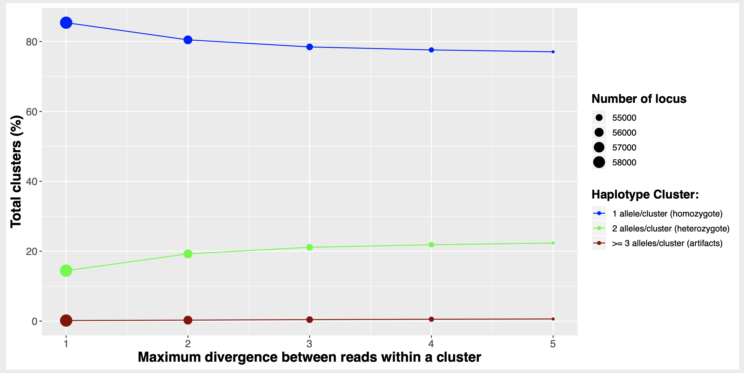
To understand this figure, I suggest you read these 2 excellent papers:

Ilut, D., Nydam, M., Hare, M. (2014). Defining Loci in Restriction-Based Reduced Representation Genomic Data from Non model Species: Sources of Bias and Diagnostics for Optimal Clustering BioMed Research International 2014(2), 1 9. https://dx.doi.org/10.1155/2014/675158

Harvey, M., Judy, C., Seeholzer, G., Maley, J. (2015). Similarity thresholds used in short read assembly reduce the comparability of population histories across species PeerJ 3(), e895. https://dx.doi.org/10.7717/peerj.895

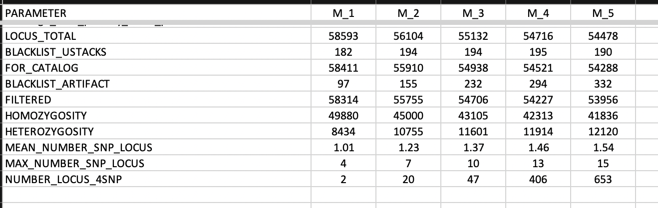
The function also produce a tibble mismatches.summary.tsv with several columns and lines summarizing ustacks output logs for the different mismatches.

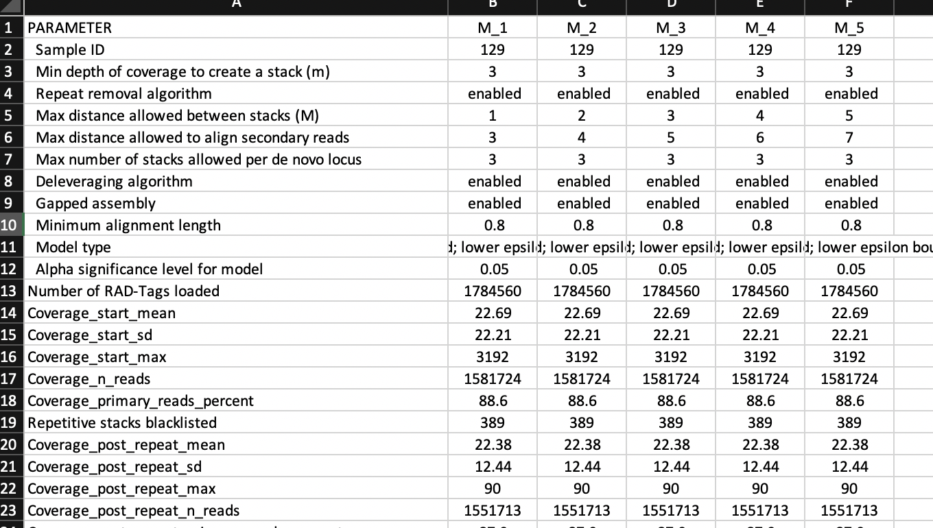
This is the data used to make the figure above.

de novo assembly

Now that you have decided the mismatch threshold, corresponding to the M argument inside stackr::run_ustacks, run the function on all samples.

Depending on project size, you might want to look at the alternative of ustacks and cstacks: run_radproc.

u <- stackr::run_ustacks(
  project.info = "02_project_info/project.info.20191121@1606.tsv",
  M = 3,
  model.type = "bounded",
  parallel.core = 12
)
# careful with the defaults...

When using paired-end data, the function uses the forward reads for the assembly. The reverse reads are used later in the pipeline.

Output:

The folder 06_ustacks_2_gstacks will be populated with 3 files per samples ending with:

alleles.tsv.gz
tags.tsv.gz
snps.tsv.gz

These files are documented here

The folder 08_stacks_results will have a summary file: summary_ustacks_date@time.tsv.

The folder 09_log_files as the associated individual log files.

run_cstacks

This is the catalog or pseudo reference genome for the de novo part of stacks, the module is called cstacks. It’s probably the longest part of the pipeline for large sample-size projects. It’s also the part where a crashing computer or cluster as the biggest drawbacks and test your bioinformatic patience.

Depending on project size, you might want to look at the alternative of ustacks and cstacks: run_radproc.

Function documentation: ?stackr::run_cstacks (read it twice).

Difference with stacks cstacks ?

Generating the catalog is split in x number of samples to make it more robust.

How?

The population map that shows which samples to use to build the catalog is split in 20 individuals (by default).
The function generates a catalog after the first 20 samples and writes it down.
cstacks starts again with the previous catalog and build a new one with new samples next on the list.
It’s incremental
Saves you a lot of time if e.g. your computer crash.
You can easily start with the catalog that was last written in the folder.

For now, I highly discourage subsampling to build the catalog = please use all the samples in the project.

Start by generating a population map:

pop.map.catalog <- u$project.info %>%
  dplyr::distinct(INDIVIDUALS_REP) %>%
  dplyr::mutate(POP_ID = 1L) %>%
  readr::write_tsv(
    x = .,
    path = "02_project_info/population.map.turtle.catalog.tsv",
    col_names = FALSE# stacks doesn't want column header
  )

Build the catalog:

c <- stackr::run_cstacks (
  P = "06_ustacks_2_gstacks",
  M = "02_project_info/population.map.turtle.catalog.tsv",
  n = 3,
  parallel.core = 32
)

Who’s in the catalog?

Use the function stackr::extract_catalog_sql_ids to verify the SQL IDs of the samples used for the catalog construction.

ids <- stackr::extract_catalog_sql_id(x = "06_ustacks_2_gstacks/catalog.tags.tsv.gz")

ustacks/cstacks alternatives ?

You have tried the noise reduction step and/or the normalization step and it’s still way to long ?

The RADProc approach developped by Praveen Nadukkalam Ravindran (Ravindran et al. 2019) is a viable alternative and it’s compatible with stacks. You replace the de novo and catalog steps by RADProc. For a project I did, it’s a question of 15 days to run stacks ustacks/cstacks or 1,5 days to run RADProc + the rest of stacks pipeline… no kidding!

Limitations

de novo only
Works only with SE RADseq data, no paired-end.
No gapped alignment (for INDELS):
- some sequencing technologies are more prone to INDEL…
- verify by generating a test set with both approach and comparing.
No control on SQL IDs (the id use for the catalog).
You cannot add sample to a pre-existing catalog: you have to start from the start with de novo assemblies of all samples you want in the catalog…

The current version works with stacks 2 (sstacks and after).

macOS installation instructions:

installing RADProc requires m4

cd Downloads
curl -O ftp://ftp.gnu.org/gnu/m4/m4-1.4.18.tar.gz
tar -xzvf m4*
cd m4*
./configure ac_cv_type_struct_sched_param=yes && make -j4 && sudo make install
cd ..
sudo rm -R m*

Download RADProc

sudo chmod -R 777 RADProc-master
cd RADProc-master/Install/
autoreconf --install
sh ./configure
make && sudo make install

Read the documentation…

To run in command line

RADProc -t "gzfastq" -f "04_process_radtags" -o "06_ustacks_2_gstacks" -M 4 -m 3 -n 4 -p 8 -x 3 -S 80 -D 7 2>&1 | tee radproc_date@time.log

To run within stackr

r <- stackr::run_radproc(M = 3, m = 4, n = 3)

Function documentation: ?stackr::run_radproc (read it twice).

The output of that command:

3 catalog files: catalog.tags.tsv, catalog.snps.tsv, catalog.alleles.tsv.
3 files per individual: tags.tsv, snps.tsv, alleles.tsv.
a file with the summary statistics.
a log file.

run_sstacks

That’s the sstacks part in stacks. It’s where the output from ustacks (the individual files) are matched against the catalog.

Function documentation: ?stackr::run_sstacks (read it twice).

Difference with stacks sstacks ?

Not much.
But I like the summary it does automatically at the end. It allows to see potential problem in the data.
Computer or server problem during the sstacks ? Just launch again the same command, the function will start again, but only with the unmatched samples!

s <- stackr::run_sstacks(parallel.core = 12)

run_tsv2bam

That’s the tsv2bam part in stacks. The tsv2bam program will transpose data so that it is oriented by locus, instead of by sample. This allows downstream improvements (e.g. Bayesian SNP calling).

If paired-end reads are available, the tsv2bam program will pull in the set of paired-end reads that are associated with each single-end locus that was assembled de novo.

Difference with stacks tsv2bam ?

after running this function, there’s no need to run SAMtools. It’s all integrated inside run_tsv2bam.
The function uses SAMtools to merge in parallel the BAM sample files into a unique BAM catalog file..

Function documentation: ?stackr::run_tsv2bam (read it twice).

# example with paired-end data:
bam.sum <- stackr::run_tsv2bam(
  M = "02_project_info/population.map.turtle.catalog.tsv",
  R = "04_process_radtags/",
  parallel.core = 12
)

run_gstacks

For some reasons, if you used paired-end data, this step won’t work for now on macOS. It’s not a stackr problem, it’s a stacks problem. Please use linux … If you don’t have access to a linux computer, try using the cloud for this step documentation.

Function documentation: ?stackr::run_gstacks (read it twice).

single-end

g <- stackr::run_gstacks(
  M = "02_project_info/population.map.turtle.catalog.tsv",
  parallel.core = 12
  )

paired-end

g <- stackr::run_gstacks(
  M = "02_project_info/population.map.turtle.catalog.tsv",
  rm.pcr.duplicates = TRUE,
  rm.unpaired.reads = TRUE,
  unpaired = FALSE,
  ignore.pe.reads = FALSE,
  parallel.core = 12
)

run_populations

For this step, I like to keep it simple and get a VCF file. Filters are best handled in my package radiator.

Function documentation: ?stackr::run_populations (read it twice).

p <- stackr::run_populations(
  M = "02_project_info/population.map.turtle.catalog.tsv", 
  verbose = TRUE, 
  r = 0.1, 
  R = 0.1,
  p = 1,
  parallele.core = 1)

Filtering

Tool: my package radiator

Missing data

Tools for visualization and imputations: grur

Population assignment

Tool: assigner

References

Rochette, N., Rivera‐Colón, A., Catchen, J. (2019). Stacks 2: Analytical methods for paired‐end sequencing improve RADseq‐based population genomics. Molecular Ecology https://dx.doi.org/10.1111/mec.15253

Ravindran, P., Bentzen, P., Bradbury, I., Beiko, R. (2019). RADProc: A computationally efficient de novo locus assembler for population studies using RADseq data Molecular Ecology Resources 19(1), 272-282. https://dx.doi.org/10.1111/1755-0998.12954

Schloss, P.D., et al., Introducing mothur: Open-source, platform-independent, community-supported software for describing and comparing microbial communities. Appl Environ Microbiol, 2009. 75(23):7537-41.

Sanders HL (1968) Marine benthic diversity: A comparative study. The American Naturalist 102: pp. 243–282

Hale et al. (2009) on the relative merits of normalization and rarefaction in gene discovery in sturgeons. BMC genomics, 10, 203.

Kalinowski (2004) Counting Alleles with Rarefaction. Conservation Genetics, 5, 539–543.

Puncher et al. (2018) Molecular Ecology Resources, 44, 678.

Using stackr to run stacks pipeline inside R/RStudio

Thierry Gosselin

2020-11-05

stackr assumptions

stackr advantages

Coding style

Workflow

Dependencies

Generate project folders

Start a project

Project info file

The art of naming your samples

single-end

paired-end

FAQ

Multiple sequencing lanes or chips ?

Technical replicates ?

No lanes just individual’s fq files ?

Transfer sequencing files

Quality control

run_process_radtags

reads length

SE RADseq

PE RADseq

QC

Noise reduction

Visualization

FAQ

Filtering ?

Data normalization

1. Wet-lab normalization

2. Bio-informatic normalization

FAQ

run_ustacks

Mismatches

de novo assembly

run_cstacks

ustacks/cstacks alternatives ?

run_sstacks

run_tsv2bam

run_gstacks

single-end

paired-end

run_populations

Filtering

Missing data

Population assignment

References