Pairwise and overall Fst with confidence intervals + building phylogenetic tree

Objectives

learn how to run the function assigner::fst_WC84
compute pairwise and overall Weir and Cockerham (1984) Fst estimates
build confidence intervals
visualize the estimates with data frame and matrices
learn how to integrate the function with other package, e.g. to build a phylogenetic tree
make Louis Bernatchez happy !

Special concerns for genome-wide estimate and filtering bias

During computation, the function first starts by keeping only the polymorphic markers in common between the populations.

When your project involves > 2 populations that evolved more by neutral processes (e.g. genetic drift) than by natural selection, filtering to keep only the markers in common between your populations will drastically reduce the number of markers, and consequently your genome coverage for the estimate. Strategically, you should reduce the threshold of number of populations required to keep a marker (e.g. use a minimum of 2 populations genotyped for the markers to keep it). This is easily tested with radiator::filter_common_markers or in stacks population module.

The overall fst and fis estimates will have reduce genome-wide coverage, because the computation is conducted with shared markers accross all your populations. However, for the pairwise comparisons, the markers will be tallied automatically for the pair. This usually results in more legitimate markers (i.e. less filtering bias) being used during computation, providing better genome-wide estimates for that pair.

Workflow

Preparation

Clean your desk and remove the clutter in the global environment

rm(list=ls())

Required libraries

if (!require("pak")) install.packages("pak")
pak::pkg_install("thierrygosselin/assigner")
library(assigner)

Get the data:

data.fst <- readr::read_tsv(file = "https://raw.githubusercontent.com/thierrygosselin/package_data/master/assigner_data_fst.tsv.gz")

Fst calculations

assigner::fst_WC84 first run: overall and pairwise, but without boostrap (i.e. no confidence intervals). Get the function documentation with: ??assigner::fst_WC84.

fst <- assigner::fst_WC84(
    data = data.fst, 
    pop.levels = c("pop1", "pop2", "pop3", "pop4", "pop5", "pop6", "pop7", "pop8", "pop9", "pop10", "pop11"),
    pairwise = TRUE,
    filename = "testing_fst", #will trigger the function to write the results in directory as well
    verbose = TRUE
)

Results

After 10 sec max you should get the Fst (overall) value of 0.05

To view the content of fst:

names(fst)

Get access to specific content with $:
- $sigma.loc: the variance components per locus: lsiga: among populations, lsigb: among individuals within populations, lsigw: within individuals.
- $fst.markers: the fst by markers
- $fst.ranked: the fst ranked
- $fst.overall: the mean fst overall markers and number of markers
- $fis.markers: the fis by markers
- $fis.overall: the mean fis overall markers and number of markers
- $fst.plot: the histogram of the overall Fst per markers
- $pairwise.fst: the pairwise fst in long/tidy data frame and number of markers per pairwise comparison
- $pairwise.fst.upper.matrix: the pairwise fst in a upper triangle matrix
- $pairwise.fst.full.matrix: the pairwise fst matrix (duplicated upper and lower triangle)
- $pairwise.fst.ci.matrix: matrix with pairwise fst in the upper triangle and the confidence intervals in the lower triangle.
To view the pairwise Fst values in a tibble with 4 columns:

df <- fst$pairwise.fst

The first 10 parwise comparisons in df

N_MARKERS: is the number of markers used between the pairs to calculate the Fst.

POP1	POP2	FST	N_MARKERS
pop1	pop2	0.0442	3457
pop1	pop3	0.0507	3457
pop1	pop4	0.0341	3457
pop1	pop5	0.0300	3457
pop1	pop6	0.0434	3457
pop1	pop7	0.0367	3457
pop1	pop8	0.0256	3457
pop1	pop9	0.0475	3457
pop1	pop10	0.0522	3457
pop1	pop11	0.0473	3457

The matrix with fst values:

# to see as a tibble:
fst.matrix <- tibble::as_tibble(fst$pairwise.fst.full.matrix, rownames = "POP")
# to keep matrix:
fst.matrix <- fst$pairwise.fst.full.matrix

If you try to get the pairwise.fst.ci.matrix:

fst$pairwise.fst.ci.matrix # you will get this:
[1] "confidence intervals not selected"

So let’s make another run with fst_WC84, but this time will ask for the confidence intervals and the heatmap:

fst.ci <- fst_WC84(data = data.fst, 
    pop.levels = c("pop1", "pop2", "pop3", "pop4", "pop5", "pop6", "pop7", "pop8", "pop9", "pop10", "pop11"),
    pairwise = TRUE,
    ci = TRUE, 
    iteration.ci = 100,
    quantiles.ci = c(0.025, 0.975),
    parallel.core = 12,
    heatmap.fst = TRUE,
    filename = "testing_fst",
    verbose = TRUE
)

`fst.ci$pairwise.fst` is the tibble with the Fst values and now with the confidence intervals.

Try again to get the matrix with fst and ci:

fst.ci$pairwise.fst.ci.matrix

To have this in a handy table for publication, we will create a new object pairwise.fst.ci.df:

pairwise.fst.ci.df <- tibble::as_tibble(fst.ci$pairwise.fst.ci.matrix, rownames = "POP")
# if you have numeric pop_id identifier you might have to do this to get proper column names:
colnames(pairwise.fst.ci.df) <- colnames(fst.ci$pairwise.fst.ci.matrix)
# to save:
readr::write_tsv(x = pairwise.fst.ci.df, path = "pairwise.fst.ci.df.tsv")

Or even better, use the heatmap of Fst and CI values…:

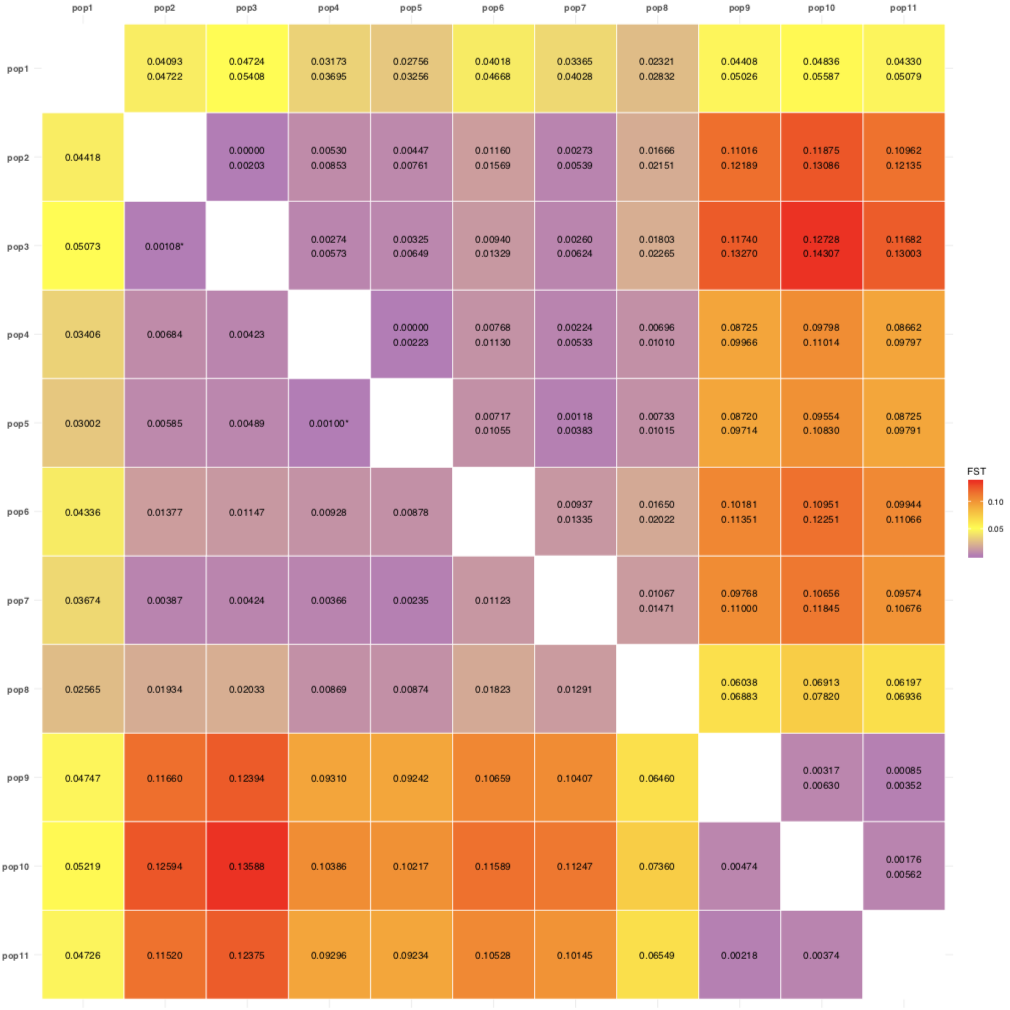
Phylogenetic tree

For the next steps, we need the full distance matrix created in step 10.

For a Neighbor joining tree:

# build the tree:
require(ape)
tree <- ape::nj(X = fst.matrix) # fst.matrix as a matrix
# for annotating bootstraps values on the tree:
bootstrap.value <- ape::boot.phylo(
    phy = tree, 
    x = fst.matrix, 
    FUN = function(x) ape::nj(x), 
    block = 1, 
    B = 10000, 
    trees = FALSE, 
    rooted = FALSE
    )
 # to get percentage values
bootstrap.value <- round((bootstrap.value/10000)*100, 0)
bootstrap.value
# to include in the tree
tree$node.label <- bootstrap.value

For a UPGMA tree:

require(stats)
tree <- ape::as.phylo(stats::hclust(stats::dist(fst.matrix), method = "average"))
bootstrap.value <- ape::boot.phylo(phy = tree, x = fst.matrix, FUN = function(xx) ape::as.phylo(stats::hclust(stats::dist(xx), method = "average")) , block = 1, B = 10000, trees = FALSE, rooted = TRUE) 
bootstrap.value <- round((bootstrap.value/10000)*100, 0)
bootstrap.value
tree$node.label <- bootstrap.value

To build the tree we will need to install

# get the latest development version of ggtree:
if (!require("ggtree")) install_github("GuangchuangYu/ggtree")
# If it's not working, use the Bioconductor version:
if (!requireNamespace("BiocManager", quietly = TRUE)) install.packages("BiocManager")
BiocManager::install("ggtree")

Several vignettes are available to get to know ggtree
Build a very basic tree figure:

require(ggtree)
require(ggplot2)
tree.figure <- ggplot2::ggplot(tree, ggplot2::aes(x, y), ladderize = TRUE) + 
    ggtree::geom_tree() + 
    # geom_tiplab(size = 3, hjust = -0.05, vjust = 0.5)+ # for just the tip label
    ggplot2::geom_text(ggplot2::aes(label = label), size = 3, hjust = -0.05, vjust = 0.5) + # for both tips and nodes
    ggtree::theme_tree() + 
    ggplot2::xlim(0, 0.16) # to allocate more space for tip labels (trial/error)
tree.figure
ggplot2::ggsave(filename = "assigner.fst.tree.example.pdf", width = 15, height = 15, dpi = 600, units = "cm", useDingbats = FALSE)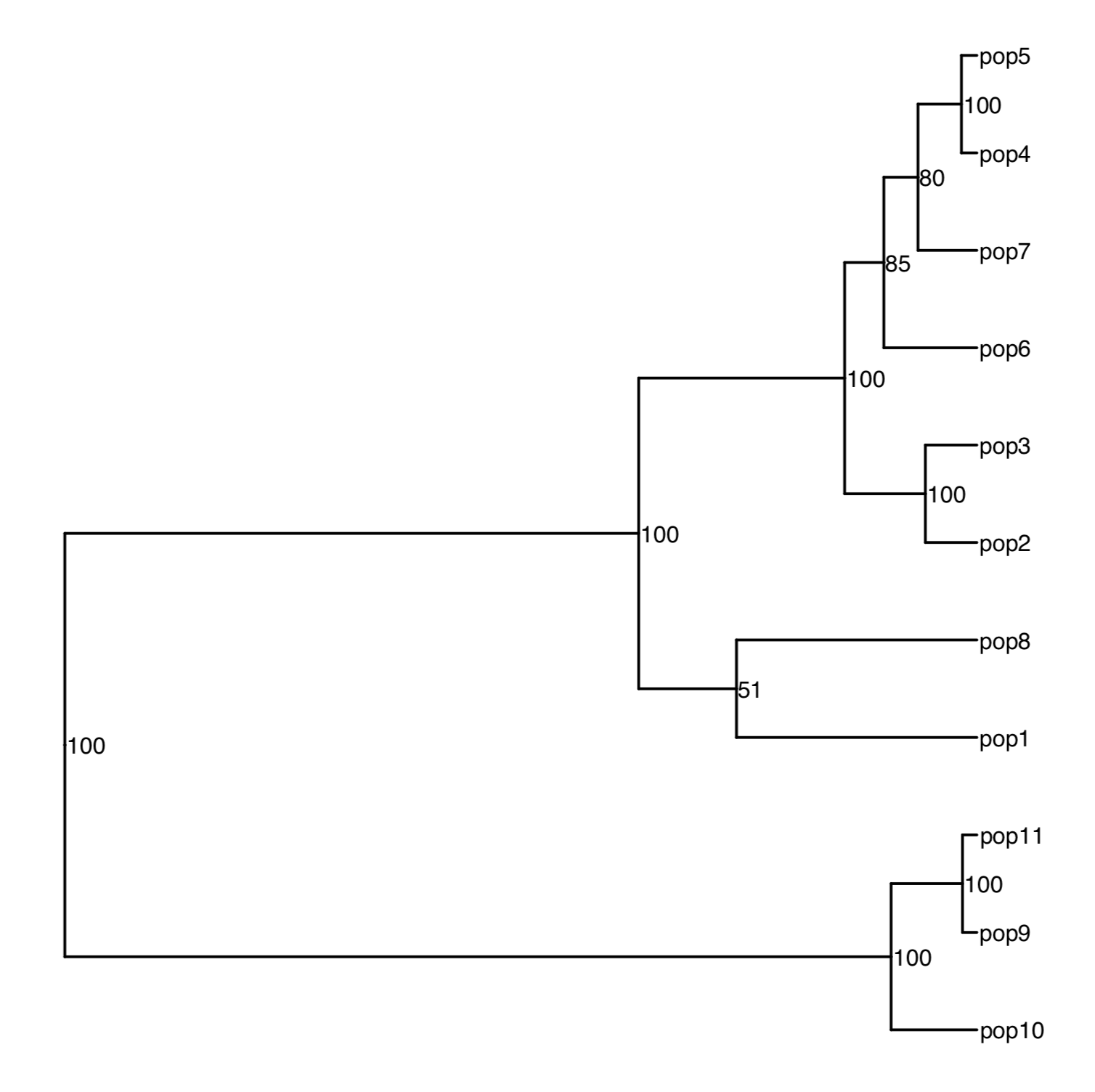

Conclusion

Please send me suggestions and bug reports through github

References

Weir BS, Cockerham CC (1984) Estimating F-Statistics for the Analysis of Population Structure. Evolution, 38, 1358–1370.

G Yu, D Smith, H Zhu, Y Guan, TTY Lam, ggtree: an R package for visualization and annotation of phylogenetic tree with different types of meta-data. revised.

Thierry Gosselin

2025-04-01