get started using assigner

Objectives

With this vignette, you should be able to learn the basics in under 30 minutes.

Assumptions:

You’ve read the function documentation on the web or with ?assigner::assignment_ngs.
You’ve read Eric’s paper: Anderson EC (2010) Assessing the power of informative subsets of loci for population assignment: standard methods are upwardly biased. Molecular Ecology Resources, 10, 701–710.
assigner is installed. If not, follow the install instructions.

Prepare your workspace

clean your workspace rm(list = ls())
load assigner

library(assigner)

By default, the working directory is where the file for this vignette is. To change: setwd("new path here")

Data 1: high structure

For this exercise, we use the first dataset included in assigner. It’s a simulated dataset generated with grur. Details of the dataset are available using: ?assigner::data_assigner_sim_01.

data <- data_assigner_sim_01

Analysis using THL with `gsi_sim`

The analysis below uses the cross-validation technique called Training, Holdout, Leave-one-out (THL):

the training of the model is conducted on 0.8 (80%) of the samples (per strata/pops)
all the markers are ranked based on Fst, only the training samples are used to generate the Fst.
the holdout samples consist of 0.2 or 20% of the samples. These are the samples assigned with gsi_sim.
the process of taking a subsample of individuals (holdout and training set) to train the model and conduct the assigment analysis with gsi_sim is repeated 5 times (iteration.method = 5).

gsi_sim is not distributed with assigner, follow the install instruction, here for my mac it’s:

assigner::install_gsi_sim(fromSource = TRUE)

no subsampling

test1 <- assigner::assignment_ngs(
  data = data,
  assignment.analysis = "gsi_sim",
  markers.sampling = "ranked", 
  thl = 0.2,
  iteration.method = 5
)
#>################################################################################
#>########################## assigner::assignment_ngs ############################
#>################################################################################
#>Execution date/time: 20190501@1104
#>Assignment analysis with gsi_sim
#>Folder created: assignment_analysis_method_ranked_20190501@1104
#>Calibrating REF/ALT alleles...
#>Subsampling: not selected
#>Conducting Assignment analysis using Training, Holdout, Leave-one-out
#>Using training samples to rank markers based on Fst
#>Holdout samples saved in your folder
#>Starting parallel computations, for progress monitor activity in folder...
#>
#>Computation time, overall: 7 sec
#>########################## assignment_ngs completed ############################

By default, the function uses all the markers and all my CPUs - 1, to change this last behavior use the argument parallel.core.

The most important information that you’ll probably want to see are both returned in the working directory and the object. Not much is kept in the object test1, because disk space is cheap, memory is not!

names(test1)
#>[1] "assignment"      "assignment.plot"

Written in the working directory under assignment_analysis_method_ranked_date@time, where date@time is the date and time the function was run:

# 01_radiator_tidy_genomic: folder
# assigner_assignment_ngs_args_20190501@1102.tsv: tibble, file
# assignment_1: folder
# assignment_2: folder
# assignment_3: folder
# assignment_4: folder
# assignment_5: folder
# assignment.plot.pdf: figure
# assignment.ranked.results.iterations.raw.tsv: tibble, file
# assignment.ranked.results.iterations.summary.tsv: tibble, file
# assignment.results.summary.stats.tsv: tibble, file
# holdout.individuals.tsv: tibble, file

These folders and files are detailed in the function documentation under value returned by the function.

To see the figure:

test1$plot.assignment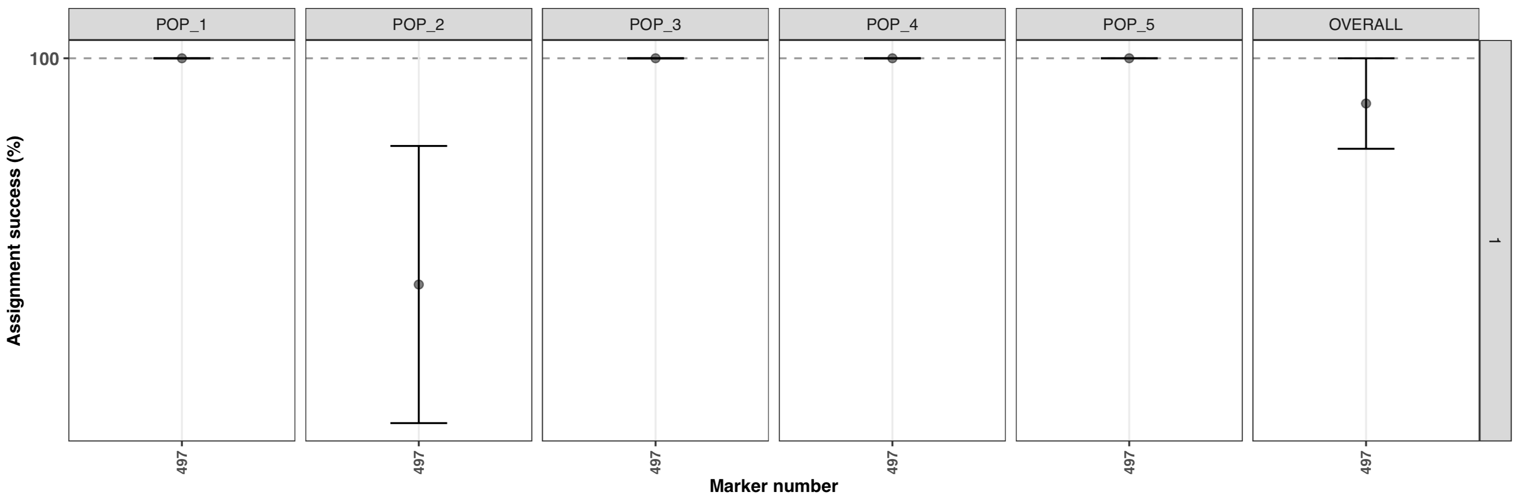

By default, the figure display the range of the data, to change this behavior and see the full range for the y axis:

test1$plot.assignment + ggplot2::scale_y_continuous(limits = c(0,100))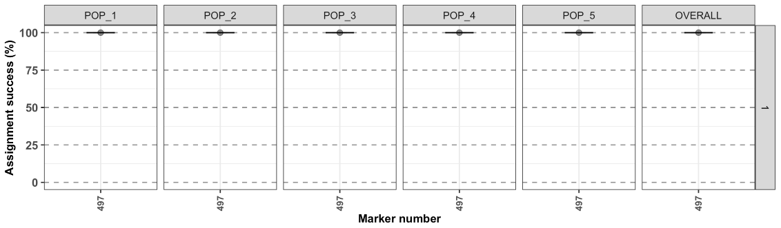

assignment is very high for all populations (the points are mean values and the error bar represent the SE based on the 5 iterations).
the horizontal facet display a 1, because subsampling of the samples was not used, only 1 set was calculated with all samples. An example below will show something different.
the x-axis display the number of marker used 497. Using dplyr::n_distinct(data$MARKERS) shows that the dataset contains 500 markers, as description of the dataset suggest, so why a lower number was used? By default, the function will keep only polymorphic markers in common between strata/pops (doc). Removing samples from the original simulated data, and low MAC result in losing 3 markers. If you want to clean the data before running the function:

data %<>% 
  radiator::filter_monomorphic(data = .) %>%
  radiator::filter_common_markers(data = .)
#>Filter monomorphic markers
#>Number of individuals / strata / chrom / locus / SNP:
#>    Blacklisted: 0 / 0 / NA / NA / 3
#>
#>Filter common markers:
#>Number of individuals / strata / chrom / locus / SNP:
#>    Blacklisted: 0 / 0 / 0 / 0 / 0

with subsampling

For the second test, we will test several marker numbers and use the subsampling arguments to select 30 individuals in each strata (repeating this 3 times).

test2 <- assigner::assignment_ngs(
  data = data,
  assignment.analysis = "gsi_sim",
  markers.sampling = "ranked", 
  thl = 0.2,
  iteration.method = 5, 
  marker.number = c(100, 200, 300, 400, "all"),
  subsample = 30, 
  iteration.subsample = 3
)
#> ################################################################################
#> ########################## assigner::assignment_ngs ############################
#> ################################################################################
#> Execution date/time: 20190501@1158
#> Assignment analysis with gsi_sim
#> Folder created: assignment_analysis_method_ranked_20190501@1158
#> Calibrating REF/ALT alleles...
#> Subsampling: selected
#>     using subsample size of: 30
#> 
#> Analyzing subsample: 1
#> Conducting Assignment analysis using Training, Holdout, Leave-one-out
#> Using training samples to rank markers based on Fst
#> Holdout samples saved in your folder
#> Starting parallel computations, for progress monitor activity in folder...
#> 
#> Analyzing subsample: 2
#> Conducting Assignment analysis using Training, Holdout, Leave-one-out
#> Using training samples to rank markers based on Fst
#> Holdout samples saved in your folder
#> Starting parallel computations, for progress monitor activity in folder...
#> 
#> Analyzing subsample: 3
#> Conducting Assignment analysis using Training, Holdout, Leave-one-out
#> Using training samples to rank markers based on Fst
#> Holdout samples saved in your folder
#> Starting parallel computations, for progress monitor activity in folder...
#> 
#> Computation time, overall: 19 sec
#> ########################## assignment_ngs completed ############################

The object generated is similar to the analysis witout subsampling. The output folder is different. The subsample folders have the same content as the output of the analysis witout subsampling.

# 01_radiator_tidy_genomic: folder
# assigner_assignment_ngs_args_20190501@1540.tsv: tibble, file
# assignment.plot.pdf: figure
# assignment.ranked.results.summary.stats.all.subsamples.tsv: tibble, file
# assignment.results.summary.stats.tsv: tibble, file
# subsample_1: folder
# subsample_2: folder
# subsample_3: folder
# subsampling_individuals.tsv: tibble, file

To view the figure:

test2$plot.assignment + ggplot2::scale_y_continuous(limits = c(0,100))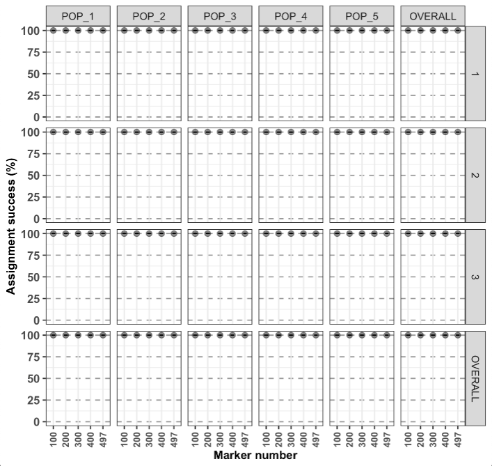

The last vertical and horizontal facets are the mean assignment for all the subsampling iterations and mean assignment over populations, respectively.
With the last plot, in the lower right corner, corresponding to the overall average (subsampling and strata/pops).
the number of markers doesn’t affect the assignment analysis, the top 100 markers are as good as using all the 497 markers. Keep in mind that this is rarely the case with real datasets…

This dataset as a high overall Fst value:

assigner::fst_WC84(data) %$% fst.overall$FST
#>[1] 0.39603

The look of the membership probabilities with adegenet dapc analysis would show something similar to this:

Data 2: low structure

Let’s try the same analysis, but this time with a dataset with lower Fst. It’s a simulated dataset generated with grur. Details of the dataset are available using: ?assigner::data_assigner_sim_02.

data <- data_assigner_sim_02

Analysis using THL with `gsi_sim`

test3 <- assigner::assignment_ngs(
  data = data,
  assignment.analysis = "gsi_sim",
  markers.sampling = "ranked", 
  thl = 0.2,
  iteration.method = 5, 
  marker.number = c(100, 200, 300, 400, "all"),
  subsample = 30, 
  iteration.subsample = 3
)

To view the figure:

test3$plot.assignment + ggplot2::scale_y_continuous(limits = c(0,100)) 
# <img src="assignment_thl_test3.png">: works
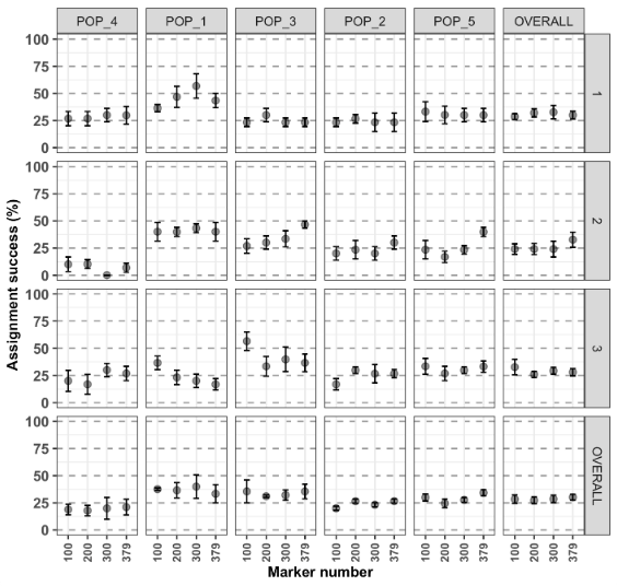#![](assignment_thl_test3.png): works
#knitr::include_graphics("assignment_thl_test3.png"):works

Very different overall results…
For the assignment analysis of species exhibiting overall low structure, using more markers will, generally, help the assingnment (if the data is filtered correctly…)

This is the overall Fst value:

assigner::fst_WC84(data) %$% fst.overall$FST
#>[1] 0.001320833

This is the membership probabilities with adegenet dapc analysis:

The populations are very admixed because of the high migration rate used during the simulations.

Analysis using LOO with gsi_sim

Let’s try using the Leave-One-Out cross-validation technique with dataset2. With this method, there is no potential bias during marker selection, you can used all the markers with marker.number = "all" or a string of marker numbers like the example above, but here, there’s no point in using less markers randomly.

The Leave-One-Out method means that the allele frequencies are calculated without the sample being assigned. This is repeated for each sample.

test4 <- assigner::assignment_ngs(
  data = data,
  assignment.analysis = "gsi_sim",
  markers.sampling = "random", 
  marker.number = "all"
)
#> ################################################################################
#> ########################## assigner::assignment_ngs ############################
#> ################################################################################
#> Execution date/time: 20190501@1317
#> Assignment analysis with gsi_sim
#> Folder created: assignment_analysis_method_random_20190501@1317
#> Calibrating REF/ALT alleles...
#> Subsampling: not selected
#> Conducting Assignment analysis with markers selected randomly
#> Making a list containing all the markers combinations
#> Starting parallel computations, for progress monitor activity in folder...
#> Summarizing the assignment analysis results by iterations and marker group
#> Compiling results
#> ########################## assignment_ngs completed ############################

To view the figure:

test4$plot.assignment + ggplot2::scale_y_continuous(limits = c(0,100))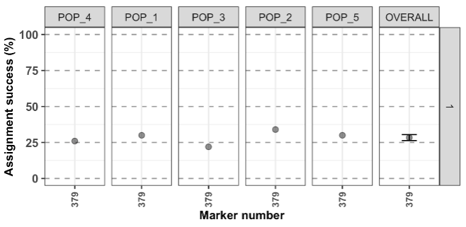

Conclusion: not much to gain here by using the LOO…

Thierry Gosselin

2023-03-15

Objectives

Prepare your workspace

Data 1: high structure

Analysis using THL with `gsi_sim`

no subsampling

with subsampling

Data 2: low structure

Analysis using THL with `gsi_sim`

Analysis using LOO with gsi_sim

get started using assigner

Thierry Gosselin

2023-03-15

Objectives

Prepare your workspace

Data 1: high structure

Analysis using THL with gsi_sim

no subsampling

with subsampling

Data 2: low structure

Analysis using THL with gsi_sim

Analysis using LOO with gsi_sim

Analysis using THL with `gsi_sim`

Analysis using THL with `gsi_sim`